The Price of Happiness

Bernoulli’s Revenge

Imagine you were given the option to play the following game: you flip a coin until it comes up heads, at which point the game ends. If you get heads on the first flip, you win $2, on the second flip, $4, on the third flip, $8. Each time you flip tails, the reward doubles, with extremely large payoffs if you manage to flip tails many times in a row before getting heads. Generically, if it takes N flips until you get heads, you’ll receive a reward of $2 raised to the Nth power, or $2^N (and if you’re the flipper, you’d like N to be as large as possible). Assuming the game can be played out instantly, what’s the most money you would be willing to pay to play this game?

One way to decide is to calculate the expected monetary value of the game, which can be easily calculated. Just multiply the value of each potential outcome by the probability that it occurs, and then add them up. But once you do that, you’ll see that the expected value approaches infinity. Why? The expected value of each flip equals the odds of getting the first heads on that flip multiplied by its payoff. Therefore, the expected value of the first flip is (50%*$2), the expected value of the second flip is (25%*$4), and so on. In other words, each flip n has an expected value of 2ⁿ / 2ⁿ = $1. Since the number of potential flips approaches infinity, the expected monetary value of this game ($1 + $1 + $1 + …) also approaches infinity. Yet would you be willing to pay your entire life’s savings to play this game, as appears to be the “rational” choice? Most people would say, “No.” Why is that?

Daniel Bernoulli attempted to solve this paradox in 1738 with a simple solution that has influenced scholarly thought ever since (1). He proposed that people don’t attempt to maximize their expected wealth, but instead attempt to maximize their expected utility. And utility, he argued, scales with the logarithm of wealth, not with wealth itself. It therefore makes sense that people are unwilling to pay an exorbitant price for a tiny chance of a large payoff, because the marginal value of money declines when you have more of it. Bernoulli’s speculation was not based on any data, as far as I’m aware. But it proposed a way to quantitatively translate an amount of money into its value to humans.

Bernoulli’s original aim with this theory was to explain why people are risk-averse. We now know that, as a theory of how humans actually make decisions, Bernoulli’s explanation is, at a minimum, incomplete. Expected Utility Theory grew out of Bernoulli’s thinking, and argued that people weight utility payoffs (rather than monetary payoffs) by their probabilities to calculate expected utility, and then make the choice that maximizes expected utility.

Kahneman and Tversky showed that Expected Utility Theory cannot account for people’s actual decisions under uncertainty, and famously proposed a different solution, Prospect Theory, they argued could explain people’s actual decisions in conditions where Expected Utility Theory failed miserably (2). Much of the revolution in decision-making research and behavioral economics over the past 40 years has built on this foundation. That research has typically sought to explain people’s real-world behavior, often by pointing out systematic inconsistencies or other deviations from apparent rationality in how people decide what to do.

At the same time, we should note something critical: the calculations that describe people’s decisions (“decision utility”) and the calculations that describe their actual utility outcomes (“experienced utility”) are not necessarily the same (3). Bernoulli’s data-free hypothesis that utility scales with the logarithm of wealth was, at least under certain conditions, quite wrong as a theory of risk-aversion (decision utility). But, as I’ll show, it appears to be exceptionally accurate as a theory describing human happiness (experienced utility). This proposition and its implications are the subject of the rest of this paper.

Money and Happiness

Few social science topics engender as much interest as the association between money and happiness. Are people who earn more money happier? Almost everyone has an opinion, even if it is based only on intuition. The research literature is large and complex, but virtually all research agrees on at least two facts: (a) the correlation between income and happiness is positive in sign; (b) the marginal value of money declines as incomes rise (4–12). In other words, richer people tend to be happier, but each additional dollar matters slightly less than the one before it. Causal evidence is much rarer, but there is compelling evidence that having more money does, on average, cause people to be happier (13–16).

In my own research, I have found that earning more money is associated with greater experienced happiness, as measured with large-scale experience sampling (17, 18). The more money people earn, the happier they tend to be in the moments of life. And this upward association appears to extend across a wide range of income levels, including well beyond a previously-accepted satiation threshold of $75,000/y. The fact that experienced happiness rises with income provides some of the most direct evidence yet that higher incomes are associated with genuinely better life experience (and genuinely better “experienced utility” in what is arguably the most literal sense we can currently measure it). A follow-up study comparing people with ordinary incomes to people with high net-worths provides extended evidence against satiation: the positive association between money and happiness appears to continue much farther, including well beyond incomes of $500,000/y, and possibly beyond the range of virtually all previous studies of money and happiness (19).

How to make sense of these findings, including my own findings as well as the broader literature, is a subject of some disagreement. Amongst researchers, educators, journalists, and laypeople, a particular issue seems especially prone to being misunderstood or overlooked: what to make of the fact that, for people’s happiness, each additional dollar appears slightly less valuable than the one before it.

After all, in our lives, we are typically used to thinking in dollars. We navigate choices quantified in dollars (or whatever one’s local currency is; here, I will refer to dollars for simplicity). But if dollars have a variable value for happiness, it’s not necessarily obvious how to approach the decisions we make with happiness in mind. Knowing well-established facts (a) and (b) noted above provide little guidance, even if one assumes that having more money really does cause people to be happier.

This Report

This report makes five key points. Collectively, they show the association between income and happiness is highly systematic, but that its implications are linear in some contexts yet exponential in others.

As is probably obvious, reasoning linearly in a situation that calls for exponential thinking, or vice versa, could lead to conclusions that are wrong. Not just a little wrong, but very wrong. For example, people sometimes assume that the diminishing value of dollars for happiness means that larger incomes have diminishing value for happiness. In my experience, this is not uncommonly asserted even by experts. While this might sound true given what I’ve said so far, it appears to be false in an important sense: as I’ll show, incomes vary exponentially in size, to a degree that appears to completely offset the declining marginal value of dollars for happiness.

Most of this paper is devoted to considering the implications of the association between income and happiness. In other words, what effects would we predict in the real-world if we extrapolate from the shape of the association? And how might our thinking need to change in different contexts? To establish a foundation for this analysis, I first show that the average trend in happiness across income levels fits Bernoulli’s theory with almost perfect precision.

This trend builds upon data on money and happiness from trackyourhappiness.org, as reported recently in other research (17–19). This includes ~1.7 million real-time reports of experienced happiness from 33,391 employed, working-age adults (ages 18 to 65) living in the United States. Participants received notifications on their smartphones at randomly-selected times during daily life, and were asked to report on their experiences at the moment just before the notification. Experienced happiness was measured with the question “How do you feel right now?” on a continuous response scale with endpoints labeled “Very bad” and “Very good.” Household income was measured with the question, “What is your total annual household income before taxes?” with answers collected in income bands. Happiness was also measured in evaluative terms via life satisfaction, including a continuous life satisfaction scale, a four-level life satisfaction scale, and the five-item seven-level Satisfaction With Life Scale (20).

Results

Point 1: The association between Log(income) and happiness was almost perfectly linear

The most common way to account for the declining marginal utility of dollars is to log transform income before correlating it with happiness. We will consider the implications of this transformation later. But first let us simply ask: how systematic is the shape of the association between happiness and Log(income)? When I previously reported this association (17) I did not calculate how well (or poorly) a linear model could explain the overall shape of the association. To quantify it, let us calculate the group-level association between Log(income) and the average happiness of the people in each income category. This averages out the substantial variation in individual happiness that income cannot explain, and isolates the underlying shape of the association between income and happiness.

Results show that Log(income) and happiness were not merely positively related. From $10,000/y to over $500,000/y, they were correlated at the aggregate level to an extremely high degree, with group-level r’s = 0.98-0.99 across a range of happiness measures, including both experienced happiness and overall life satisfaction, see Fig. 1. These group-level correlations remain high when controlling for demographic variables (age, gender, education level, and marriage), r’s = 0.95-0.99.

Fig. 1. Mean levels of happiness, including experienced happiness (real-time feelings) and overall life satisfaction, for each income category. The group-level correlations between happiness and Log(income) is displayed. Income axis is log scaled, and error bars indicate 95% confidence intervals. Because the top 3 income categories have progressively fewer people and progressively wider confidence intervals, a composite point (displayed in gray) that combines them and is comparable in size to the other income categories is also plotted for reference (it is not included in the correlation or fit line calculations).

In other words, the average happiness of people in each income category was almost perfectly linearly associated with that category’s Log(income), explaining virtually 100% of group-level variation. This is just as Bernoulli’s nearly 300-year-old theory predicts, if we extend it from wealth to income and from “decision utility” to happiness.

When explaining how happiness varies between income levels, a linear prediction from Log(income) was superbly accurate¹. If we assume this remarkably systematic shape indicates the “price of happiness”, what are the implications for the rest of human life?

Point 2: This entails a diminishing marginal value of dollars, but shouldn’t be confused with a plateau

If happiness rises linearly with Log(income), it implies that the marginal value of a dollar diminishes exponentially, at least in terms of predicting happiness. For example, an extra $10,000 would be expected to “matter” much more to happiness for a person earning $25,000/y than a person earning $200,000/y, and it would be expected to take ever-greater increments of income to achieve the same increment in happiness as incomes rise. When the association between happiness and income is plotted on a linear axis instead of a logarithmic axis, the declining marginal value of a dollar is clear (see Fig. 2).

Fig. 2. Estimated levels of happiness plotted as a linear function of Log(income), which Figure 1 shows fit the data extremely well. Income axis is linear, not log transformed.

The declining marginal value of a dollar is no more or less true when plotted on a linear axis, of course, but plotting it this way makes its truth obvious. The shapes observed in Fig. 1 and Fig. 2 are equivalent to each other and are equally correct. The problem is that Fig. 2 can be misleading. While it might seem that this curve is asymptotic and will quickly reach a maximum value for happiness beyond which additional income makes no difference, a mathematically linear relationship between happiness and Log(income) is, in reality, not asymptotic. It will never reach a plateau. There may well be some income threshold in the real world beyond which happiness fails to increase, but the point to recognize here is that the existence of a plateau is not predicted mathematically by a logarithmic association.

For example, one might look at Fig. 2 and conclude that beyond $400,000/y more money makes very little difference, but if we extrapolated the same fit line to a much higher income range and plotted happiness for incomes ranging from $500,000/y to $15 million/y, one might then be tempted to conclude with equal confidence that more money matters, but that beyond $10 million/y more money makes very little difference².

Additionally, proportional differences in income would be predicted to have a constant and non-diminishing association with happiness. For example, a 10% difference in income would be associated with exactly the same difference in happiness, regardless of income level. See the Appendix for an extended explanation and a brief review of the math of logarithms applied to income and happiness.

Anytime one plots an exponential relationship on a linear axis there can appear to mathematically-naive eyes to be an impending plateau. But the point at which a plateau appears to begin is arbitrary. We simply cannot trust our intuitive sense that a plateau is impending when underlying variation is exponential.

Is the world flat or curvy?

How should one make sense of these two patterns? If happiness varies linearly with Log(income) and we want to extrapolate from that association to make predictions for the real-world (whether purely descriptive predictions or, in some cases, causal predictions), how should we conceptualize the association between happiness and income? As a flat line as in Fig. 1, or an exponentially diminishing curve as in Fig. 2? Is income, and money more generally, something whose implications for happiness would be predicted to diminish exponentially, or stay constant, in real-world decisions? The answer appears to be: Both, but in different contexts. Let us examine them in turn.

Point 3: Individual incomes differed exponentially in size, offsetting the declining marginal value of dollars. As a result, larger real-world incomes were associated with non-diminishing increments in both Log(income) and happiness.

Perhaps the most obvious reason to be interested in the shape of the association between income and happiness is to know whether larger incomes have diminishing returns for happiness, or not.

If dollars get exponentially less valuable when you have more of them, one might assume that the benefits of a larger income also diminish rapidly, even if no true plateau is reached. Indeed, this is a common assumption when people notice happiness plotted against a logarithmic income axis.

But this assumption depends on an entirely separate feature of reality that is sometimes not considered: How the sizes of incomes vary in the real-world.

So what does the distribution of real-world incomes look like? One possibility is that values of Log(income) differ mainly at the lower end of the income distribution, with comparatively little differentiation amongst high earners. If this were true, we might reasonably expect that most of the room for happiness to rise with income is at the lower end of the income distribution. A second possibility is that incomes themselves differ exponentially in size and that values of Log(income) differ just as much at the high end of the income distribution as at the low end of the income distribution. If that were true, we would not have reason to expect a decline in the marginal utility of a larger real-world income.

Evidence strongly favored the latter possibility. If we rank people in order of income, we can view income levels based on their position in the income distribution. A plot of income across 20 income quantiles reveals that the value of Log(income) increases just as steeply across high incomes as low incomes (r = 0.98, see Fig. S1). Data on incomes from the U.S. Congressional Budget Office show a virtually identical income distribution (see Fig. S2), showing that this pattern reflects a realistic income distribution, not something idiosyncratic to this sample of people.

Now the real question: Does the association between happiness and one’s position in the distribution of real-world incomes (income quantile) look more like Fig. 1, or more like Fig. 2? Is it consistent with diminishing marginal value of a larger income, or not?

The results are clear. Income quantile had a linear association with happiness (see Fig. 3). As a result, it’s possible to reproduce the linear relationship observed between income and happiness without a logarithmic transformation. All one needs to do is plot a person’s position in the real-world income distribution. The group-level correlation between income quantile (range: 1 to 20) and mean experienced happiness for each quantile is r = 0.96, with a highly linear shape. The results are comparably linear for the three life satisfaction measures (r = 0.98-0.99). This pattern is consistent with the possibility that moving up to the next highest income in the real-world would have the same relationship to happiness, regardless of one’s position in the distribution of incomes. For example, it suggests that a higher-paying occupation or job would be associated with similar gains to happiness regardless of income level (at least within the range of incomes observed here)³.

Fig. 3. Mean levels of happiness, including experienced happiness (real-time feelings) and overall life satisfaction, across 20 income quantiles. The group-level correlations between happiness and income quantile is displayed.

These results collectively show that income itself varies exponentially in size across the income distribution, to such a degree that it counteracts the exponentially diminishing marginal value of money when it comes to predicting happiness. Each step up the ladder of real-world incomes was associated with a non-diminishing increment in Log(income) and a non-diminishing increment in happiness.

The concavity one sees when plotting income on a linear axis (as in Fig. 2) can therefore be doubly misleading: not only does it appear to suggest the possibility of an asymptote or plateau in happiness when none exists mathematically, but it also fails to capture the exponentially growing sizes of people’s incomes.

Point 4: Exponential differences in happiness are predicted in other domains, including large financial risks and trade-offs between people with unequal incomes.

The preceding analysis shows that, despite the exponential decline in the marginal value of a dollar for happiness, individuals nevertheless exhibit a linear, non-diminishing association between larger real-world incomes and greater happiness. The same would be predicted for proportional variation in income, such as a 5% change in income for an individual, or a 5% change applied equiproportionately to a population (10). Yet that pattern does not apply to every context. There are other contexts where the declining marginal utility of money would indeed be expected to have exponential implications.

Let us assume for the sake of following hypothetical examples that (i) the association between happiness and Log(income) is linear across the entire range of possible incomes (including incomes higher and lower than those observed here), (ii) the association reflects a causal relationship where more money produces greater happiness, (iii) we are only modeling the effects of income on happiness (ignoring all other considerations for simplicity), and (iv) units of reported happiness represent the same amount of happiness, on average, at different income levels. Although we will assume the sign (positive) and shape (linear) of the relationship, we do not need to assume anything about its magnitude: Everything that follows is independent of the magnitude of the alleged effect of money on happiness. Some of these assumptions are likely to be violated to some extent in the real-world, of course, but contemplating a version of the world where they are precisely true makes it possible to explore the implications of a linear association between happiness and Log(income).

One individual context where the exponential decline in the marginal value of dollars for happiness could be important are high-stakes risky bets. This takes us back to the type of scenario Bernoulli contemplated in 1738 when he speculated that utility scaled with the logarithm of wealth (1), even though at the time he was focused on explaining people’s risk-averse behavior (at which his theory ultimately fares poorly (21)), rather than predicting their happiness (at which his theory appears to fare remarkably well).

Consider a hypothetical person who has permanently retired with a pension of $50,000/y and has no other income or savings. If this person is given the choice between two options: a “safe option” with a 100% chance that their income doubles to $100,000/y, and a “risky option” that has a 90% chance of failure (their income remains $50,000/y) and a 10% chance of success and a larger payoff. How big does the risky payoff need to be to equate its expected value for happiness?

One’s first instinct might be to assume the risky payoff needs to be ten times as large at $500,000/y (plus the original $50,000/y). But that is not nearly enough. This equates the expected value in dollars ($100,000/y), but it doesn’t come anywhere close to equating the expected value for happiness. To achieve parity with a guaranteed income of $100,000/y, the risky payoff with a 10% chance of success would have to be approximately $50,000,000/y!

Why is this? Each additional dollar is exponentially less valuable, so a lot more money is needed. To match the predicted happiness associated with the safe option (the guaranteed doubling of income) with a 10% chance of a bigger payoff, the risky payoff would need to be 2¹⁰ = 1,024 times current income, or over $50,000,000/y. The reason is that equating the expected utility of the safe and risky payoffs requires the following:

100% * Log(2) = 10% * Log(risky payoff)

…which is only true if the risky payoff is 2¹⁰ times current income. If the risky option had a 50% chance of success, the risky payoff would need to be a more modest 2² times current income, or $200,000/y (a $150,000/y increase). If the risky option had only a 1% chance of success, the risky payoff would need to be 2¹⁰⁰ times current income, or far more than all money in circulation, to achieve parity for happiness. Exponential indeed. Working for many years at a risky start-up at a low salary or spending money on lottery tickets may be even less rational than they appear, if we are willing to reduce the calculation to the pattern described here.

If we consider risks in the domain of losses instead of gains, the same simple relationship shows why insurance could be expected to be beneficial for happiness when the downside risk is very large. If a person risks losing a substantial fraction of their total lifetime earnings (such as in the case of a house fire or permanent disability), then even insurance sold at a price profitable to an insurer (i.e., with a negative expected monetary value for the consumer) could be quite beneficial to the consumer’s well-being (i.e., with a positive expected value for happiness). In such cases, insurance premiums are purchased with exponentially less valuable dollars than the dollars against whose loss they protect against.

The fact that insurance can be justified by declining marginal utility is not at all a new point, of course - it is a fundamental rationale of insurance against major risks. In fact, it is a mathematical consequence of a logarithmic utility curve that Bernoulli himself explored in his 1738 paper. However, the present results suggest it could potentially be justified and calculated from real-world happiness data, as opposed to theoretical assumptions about an opaque conception of utility.

However, there’s another important context to consider. Exponential differences are especially apparent, and perhaps most consequential, in situations that involve trade-offs between people with very different incomes. If dollars become exponentially less valuable as incomes rise, then the well-being benefits of a given dollar are predicted to be exponentially larger for a poorer person than a richer person.

Take philanthropy. Let us assume that money can be efficiently invested to improve the lives of people who are poor on the global scale (e.g., earning $2/day), and that there is a 1:1 monetary cost:benefit ratio. Perhaps money could be used to invest in health care, nutrition, education, or job training, or simply delivered directly via unconditional cash transfer. This hypothetical example simply assumes $1 of benefit to the beneficiary’s income for each $1 invested without regard to mechanism. Under these assumptions, a dollar contributed by a person earning $73,000/y that increases the income of a person earning $2/day ($730/y) would generate a predicted ROI of approximately 10,000% for happiness⁴. Why? Because their earnings differ by a factor of 100, the benefit to happiness of that dollar is estimated to be 100 times greater for the person earning $2/day than the loss incurred by the person earning $73,000/y (for an experimental test of a similar idea, see (14)).

What if we take the example to the extreme and consider a hypothetical superwealthy person who earns $1 billion/y and decides to voluntarily contribute to people earning $2/day, under otherwise identical assumptions (since we are only modeling the effects of income, for simplicity let us assume this person has a very large income stream and ignore wealth). Now, the predicted ROI of the first dollar is nearly 137,000,000%! Or to play out a more complete example, the billionaire contributing 10% of her income to double the incomes of people earning $2/day would be expected to generate ≈ 90,000,000% return on investment for collective human happiness⁵. No investor could ordinarily achieve a 90,000,000% rate of return on such a large amount of money. If they did, it would mean turning that $100 million into over $90 trillion in one year’s time, an amount approximately equal to the entire world’s GDP in 2021.

The same logic could extend to many other situations. For example, decision-makers that seek to improve collective happiness might find that preferentially increasing incomes of those who earn the least generates a large ROI for collective happiness. In the domain of compensation, an employer allocating marginal dollars to raise the incomes of employees earning $30,000/y is predicted to generate 20x (2,000%) as much marginal happiness as raising the incomes of employees earning $600,000/y, and 200x (20,000%) as much marginal happiness as raising the incomes of employees earning $6,000,000/y. Organizations sometimes do just the opposite, paying large bonuses to highly-paid executives rather than directing discretionary compensation to the people on whom it would be expected to have the largest impact. Similarly, nations sometimes apply relatively low tax rates on their richest citizens, even though money appears to be exponentially more important to the well-being of those who earn less.

The above numbers and predictions are based on simplistic assumptions that are sure to be violated to at least some extent in the real world, of course. In practice, ROI values could be larger or smaller than calculated here, or even backfire and become negative in some cases. And in dynamic systems like an economy or a society, long-term consequences can be hard to predict even when short-term effects are known. Needless to say, accurate predictions of the consequences of any specific action lies far beyond the scope of this paper. The point is not the precise values but, instead, the simple observation that there are large and calculable implications of a linear relationship between happiness and Log(income) when trade-offs are made between people with unequal incomes, and that these mathematical implications can play out quite differently than they do for an individual person navigating different income levels.

In the most prominent cases involving money and happiness, the world is flat (like Fig. 1) for people making individual decisions, but the world is curvy (like Fig. 2) for people making collective decisions.

Point 5: Money’s diverging implications for happiness, linear in some contexts but exponential in others, could help explain why income inequality persists as societies get richer, why the income distribution is shaped the way it is, and why happiness in the U.S. has not seen more improvement in recent decades.

Consider a world quite different from the one we appear to inhabit. If, contrary of the pattern described here, the payoff of a higher income for individual happiness (i.e., its marginal utility) did exponentially diminish, then we would have some reason to expect a trend towards greater income equality over time if a society becomes richer. Why? For a well-off individual in that hypothetical world, there would be less and less to gain from a higher income and it would make sense progressively deprioritize a higher income relative to other priorities, at least from the standpoint of happiness. If such a society got richer over time, there would be some reason to expect this to disproportionately raise the bottom of the income distribution as low earners seek to improve their financial lot and, accordingly, their happiness, leading to ever-decreasing income inequality. This suggests the potential for a harmonious relationship between individual and collective happiness in relation to money, since the pursuit of individual and collective happiness would tend to converge as a society got richer. But that does not appear to be the reality we live in, at least within the range of incomes observed here.

In actual reality, the expected payoff of a larger real-world income for happiness appears to remain approximately constant, on average, such that it could be entirely reasonable for an individual to continue aspiring to climb one more rung in the income ladder, if all else is held equal. But since each rung entails exponentially more dollars, the successful pursuit of higher incomes for the well-off could perpetuate inequality, as large quantities of money are allocated to a small group of people who succeed in becoming richer. This could be suboptimal for collective happiness if increases to a large income are achieved primarily through value capture (capturing a bigger slice for oneself without growing the size of the pie) rather than primarily through value creation (getting a bigger slice by creating a bigger pie). When it comes to money, this highlights a potential tension in the geometry of individual and collective happiness.

This pattern of results might also help explain why incomes differ exponentially in size in the first place. For example, larger incomes incentivize people to take certain jobs over others, to seek promotions, and to be productive. If happiness varies linearly with Log(income), then to achieve a non-diminishing incentive, incomes might need to grow exponentially larger in size. If they didn’t, the power of money as an incentive (at least in terms of happiness) would diminish dramatically. Some people would surely still choose to be CEOs even if they didn’t earn millions of dollars. But to the extent that a market economy uses money to incentivize behavior, the pattern described here offers a potential explanation for why salaries differ so greatly in size: they vary exponentially in order to maintain a non-diminishing association to happiness. After all, even if human decision-making is subject to a host of quirks and irrationalities, it is affected by incentives, too. This tendency might be accentuated if high-paying jobs also have a larger component of variable compensation (recall the “risky payoff” calculations).

Finally, this pattern could at least partly explain a puzzle: happiness in the U.S. has stagnated in recent decades despite growing GDP per capita (22, 23). One contributing reason could be that income growth has been disproportionately concentrated at the top of the income distribution. In recent decades, it’s the highest earners in the U.S. who have experienced the fastest income growth, even in percentage terms (they have gained exponentially more, in dollar terms). In contrast, real (i.e., inflation-adjusted) incomes for lower income folks, where additional dollars would be expected to have an exponentially larger impact on happiness, have grown the slowest for decades (24). This is precisely opposite to the trend these results predict would most benefit a society’s collective happiness. Setting aside the countless complexities that the present model does not account for, if income growth is going to be unequally distributed, these results predict that society’s average happiness would benefit the most if economic growth disproportionately benefited the poorest people instead of disproportionately benefiting the richest. Alternatively, equiproportionate gains, with the same percentage increase throughout the income distribution, would evenly distribute the expected happiness benefits of economic growth.

Discussion

Understanding the association between income and happiness has the potential to help us make decisions that support human well-being. While the association between income and happiness is one of the most studied topics in the happiness literature, it is common even for researchers to disagree about what it means for happiness to vary with Log(income), and sometimes even to disagree about the appropriateness of log-transforming income in the first place (for instance, I have heard at least one highly influential researcher describe the transformation itself as a “sleight of hand”).

These results suggest that the association between income and happiness is extremely systematic. The aggregate association between happiness and income was characterized almost perfectly as a linear association with Log(income), with group-level r’s = 0.98-0.99 across a range of happiness measures. This shows remarkable agreement with Bernoulli’s formulation in 1738, albeit in a different sense than he intended. While the linear relationship to Log(income) predicts an exponential decline in the marginal value of a dollar, it also predicts that proportional differences, such as a 10% increase, would be associated with the same difference in happiness regardless of income level.

One might assume that the exponential decline in the marginal value of money means that most variation in happiness occurs in the lower income range. One might also assume that income effectively stops mattering in practical terms for happiness beyond some modest income threshold, even if the slope with Log(income) technically remains positive.

This report suggests that both of these assumptions are wrong in an important sense. The sizes of incomes increased exponentially across the income distribution, to such a degree that the association between happiness and a person’s position in the income distribution was highly linear (r = 0.96-0.99), even without a logarithmic transformation. In the end, traversing the space of possible incomes (e.g., by choosing one occupation over another, or one job or another) is predicted to result in non-diminishing differences in happiness, on average, across a wide range of income levels.

On the other hand, in the domains where decisions can entail trade-offs between people with highly unequal incomes, such as philanthropy, tax policy, compensation decisions, and others, the exponentially diminishing value of dollars for happiness does predict exponential consequences. For example, a person would be predicted to generate astronomical returns for collective happiness if they could effectively invest a fraction of their income to improve the lives of people who are very poor. An employer could do the same by giving discretionary bonuses to the lowest paid workers instead of giving them only to the highest earners. Likewise, if gains from economic growth are shared throughout the income distribution, rather than mainly benefiting the well-off, it might greatly amplify the benefit of economic growth for a society’s well-being. Finally, high-stakes financial risks also yield exponential predictions, even at an individual level.

Knowing when to think linearly and when to think exponentially is crucial for understanding the relationship between money and happiness.

Footnotes

^{1. It’s worth noting that the highly linear shape is revealed when averaging across people, but of course that doesn’t tell us what the shape would be for a specific person. The linear shape is a sensible starting point for individual predictions, but a given individual could ultimately follow a somewhat different shape in reality. We just know that the cross-sectional average of those shapes is extremely linear.}

^{Additionally, the highly linear shape reported in this paper describes the association between Log(income) and happiness, but can’t directly reveal the shape of the causal relationship. There is strong evidence that having more money does indeed cause higher happiness, as noted in the introduction, and given the strikingly linear shape of the association it is quite plausible that the causal relationship is also linear, but the field currently lacks definitive data on the nuanced shape of the causal relationship itself. Some of the implications discussed in this paper address the question: if the causal relationship follows the same shape as the cross-sectional association, what would the implications be? Further research would be needed to test this proposition explicitly.↩}

^{2. The same is true in reverse for exponential growth. Consider a hypothetical bacterial colony with unlimited space and food that doubles in size every 6 hours. No matter how long the growth period, if the number of bacteria is plotted on a linear axis, it will seem as if nothing happens until the last few days. But there is nothing special about a given number of days, and it takes a logarithmic axis to reveal the true pattern of growth.↩}

^{3. While this explanation interprets the result as if Log(income) is the key predictor, one might alternatively wonder whether it is relative income (i.e., income rank) that is actually the key predictor. It is likely that both relative and absolute income matter, but relative income seems unlikely to explain all or even most of the relationship between money and happiness. There are a few reasons for this, but a prominent one relates to a nation’s happiness and its association with income (5, 10). If happiness were determined entirely by one’s income relative to those in physical or psychological proximity, then we would have reason to expect a relatively steep income:happiness gradient within-nations (or within a given person’s reference group) and, by comparison, a relatively weak gradient between-nations (or between different people’s reference groups). In reality, not only is there a substantial income:happiness association between nations, but the slopes of happiness:Log(income) within-nations and between-nations are virtually identical in magnitude (e.g., see Figs. 11-12 in (10)). While well-being may be sensitive to relative income to some degree, the aforementioned evidence is consistent with a large role for absolute income and a limited role (or perhaps no net role at all) for relative income. At the same time, there is no straightforward and definitive answer for why money and happiness are related, and the forces underlying the relationship are likely to be complex, even if the average trend is simple.↩}

^{4. Technically, the ROI would be 9,900% once we subtract the loss incurred by the donor.↩}

^{5. Why is the ROI ≈ 90,000,000%? Because 136,986 people would see their incomes double, in exchange for a 10% reduction for one person. Since the logarithmic math predicts that each beneficiary gains 6.58 times as much well-being as the single donor loses (log(2) / log(0.9)), we can multiply the 6.58 benefit:cost ratio by the 136,986 beneficiary:donor ratio to arrive at an approximate ROI estimate.↩}

Cite this

Killingsworth, M. A. (2024). The Price of Happiness. Happiness Science. https://happiness-science.org/price-of-happiness

References

1. D. Bernoulli, Specimen theoriae novae de mensura sortis. Commentarii Academiae Scientiarum Imperialis Petropolitanae 5 (1738).
2. D. Kahneman, A. Tversky, Prospect Theory: An Analysis of Decision under Risk. Econometrica 47, 263 (1979).
3. D. Kahneman, P. P. Wakker, R. Sarin, Back to Bentham? Explorations of Experienced Utility. The Quarterly Journal of Economics 112, 375–406 (1997).
4. M. Argyle, “Causes and correlates of happiness” in Wellbeing: The Foundations of Hedonic Psychology, D. Kahneman, E. Diener, N. Schwarz, Eds. (Russell Sage Foundation, 1999), pp. 353–373.
5. A. Deaton, Income, Health, and Well-Being around the World: Evidence from the Gallup World Poll. Journal of Economic Perspectives 22, 53–72 (2008).
6. E. Diener, R. Biswas-Diener, Will money increase subjective well-being? Social indicators research 57, 119–169 (2002).
7. D. Kahneman, “Objective Happiness” in Well-Being: Foundations of Hedonic Psychology, D. Kahneman, E. Diener, N. Schwarz, Eds. (Russell Sage Foundation, 1999), pp. 3–25.
8. D. Kahneman, A. Deaton, High income improves evaluation of life but not emotional well-being. Proceedings of the National Academy of Sciences of the United States of America 107, 16489–93 (2010).
9. R. Layard, S. Nickell, G. Mayraz, The marginal utility of income. Journal of Public Economics 92, 1846–1857 (2008).
10. B. Stevenson, J. Wolfers, Economic growth and subjective well-being: Reassessing the Easterlin Paradox. Brookings Papers on Economic Activity 2008, 1–87 (2008).
11. B. Stevenson, J. Wolfers, Subjective Well-Being and Income: Is There Any Evidence of Satiation? American Economic Review 103, 598–604 (2013).
12. R. Veenhoven, M. Hagerty, Rising Happiness in Nations 1946–2004: A Reply to Easterlin. Social Indicators Research 79, 421–436 (2006).
13. J. Gardner, A. J. Oswald, Money and mental wellbeing: A longitudinal study of medium-sized lottery wins. Journal of Health Economics vol, 26pp49-60 (2007).
14. R. J. Dwyer, E. W. Dunn, Wealth redistribution promotes happiness. Proceedings of the National Academy of Sciences 119 (2022).
15. S. Kim, A. J. Oswald, Happy Lottery Winners and Lottery-Ticket Bias. Review of Income and Wealth 67 (2021).
16. E. Lindqvist, R. Östling, D. Cesarini, Long-Run Effects of Lottery Wealth on Psychological Well-Being. The Review of Economic Studies 87, 2703–2726 (2020).
17. M. A. Killingsworth, Experienced well-being rises with income, even above $75,000 per year. Proceedings of the National Academy of Sciences 118, e2016976118 (2021).
18. M. A. Killingsworth, D. Kahneman, B. Mellers, Income and emotional well-being: A conflict resolved. Proceedings of the National Academy of Sciences 120 (2023).
19. M. A. Killingsworth, Money and Happiness: Extended Evidence Against Satiation. Happiness Science (2024).
20. E. Diener, R. A. Emmons, R. J. Larsen, S. Griffin, The Satisfaction With Life Scale. Journal of Personality Assessment 49, 71–75 (1985).
21. D. Kahneman, Thinking, Fast and Slow (Farrar, Straus and Giroux, 2011).
22. D. Blanchflower, A. Oswald, Well-being over time in Britain and the USA. Journal of public economics (2004).
23. B. Stevenson, J. Wolfers, The paradox of declining female happiness. American Economic Journal: Economic Policy 1, 190–225 (2009).
24. U.S. Census Bureau, Historical Income Tables: Households. Census.gov. Available at: https://www.census.gov/data/tables/time-series/demo/income-poverty/historical-income-households.html [Accessed 7 December 2023].

Appendix

The income distribution

Fig. S1 The distribution of Log(income) across 20 income quantiles. Note that the x-axis is income quantile, and the y-axis is Log-scaled income. While the underlying shape is not perfectly linear, a linear fit can nevertheless explain it quite well (r = 0.98).

Note that while the correlation in Fig. S1 is very high (r = 0.98), the curvature in the tails is consistent with a normal distribution of income in logarithmic/exponential space, rather than a precisely linear relationship (i.e., a uniform distribution). The relevant point for this paper is that the distribution is approximately symmetrical, and increases just as quickly on the high end as the low end. But Log(income), and potentially happiness, do show faster change in the tails, especially the top and bottom 5%.

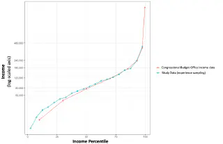
Fig. S2 Household income distribution according to the Congressional Budget Office (2018 data, before taxes and transfers) compared to the distribution of incomes in the current study across 20 quantiles (as also shown in Fig. S1). CBO data is available by quintile for the first four quintiles and then in smaller quantiles within the top quintile.

Modeling the association between income and happiness

Let us take a moment and clarify the quantitative form of the association between income and happiness. The very high aggregate correlation (group-level r’s = 0.98-0.99, across a range of measures) shows that the aggregate variation in happiness that is explained by income can be modeled almost perfectly with the following standard formula:

happiness = k + b * Log(income)

Formula 1. The linear relationship between happiness and Log(income).

A complete understanding of the real-world relationship between income and happiness, especially for any specific individual, requires answering both general and idiosyncratic questions about the magnitude of the causal effect, effect moderators, earnings history, expectations for the future, reference groups, and countless other complexities. Moreover, past or future research could argue against a perfectly linear relationship between happiness and Log(income) across all possible income levels. Finally, as incomes rise it is also likely that a greater share of a person’s total financial resources may take the form of wealth in addition to income.

While this complexity is worth acknowledging, this report aims to set this complexity aside for most of its analysis, and instead asks: if we assume that Formula 1 correctly models the average shape of the relationship that exists between income and happiness over a relevant range of incomes, what are the implications?

The implications of this association are important to understand but not necessarily obvious. The mathematical implication of Formula 1 is that the marginal utility of income diminishes exponentially, while the marginal utility of proportional difference in income (such as a 10% difference) is constant and does not diminish. Why is this the case?

Imagine we wanted to calculate the difference in predicted happiness for two people, person_a and person_b, based on the difference in their incomes (income_a and income_b), or the difference in predicted happiness for two different income levels for the same person (say, after versus before a salary increase, again represented as income_a vs. income_b) using Formula 1. The difference in predicted happiness would be linearly related to the difference in Log(income).

Δ Happiness_{a – b} = Happiness_a – Happiness_b

= k + b * Log(incomea) – (k + b * Log(income_b))

= b * (Log(income_a) – Log(income_b))

The difference in predicted happiness for two incomes is a linear function of the difference in Log(income). But there’s a further simplification we can make: the logarithm of a quotient is equal to the difference of the logarithms. In other words, Log(a/b) = Log(a) – Log(b). As a result, we can simplify the calculation of the difference in happiness for two incomes as:

Δ Happiness_{a – b} = b * Log(income_a / income_b)

Formula 2. Happiness varies logarithmically with the ratio of two incomes.

With this simple formula in mind - a formula that is no doubt already familiar in form to some psychologists and to many economists - it is clear why the marginal value of money declines, while the marginal value of a proportional difference is constant.

The math is simple: Log((income +1) / income) will get smaller as income increases in size, showing that the marginal value of a unit of currency declines as incomes rise. Yet Log((income*1.1) / income) will remain constant as income increases in size, because the value of income drops entirely from the calculation. Log((income*1.1) / income) is simply equal to Log(1.1), showing that the marginal value of a proportional difference in income is predicted to be constant, regardless of one’s absolute level of income. According to Formula 2, the expected effect of a proportional difference in income does not depend on one’s income level.

Materials and Methods

Sample information. Participants were 33,391 employed adults living in the U.S. Median age was 33, median household income was $85,000/year, 36% were male, 37% were married. To reduce confounding effects on the association between income and happiness such as unemployment, retirement, and family income transfers, participants were restricted to employed adults living in the U.S. of working age (18-65) who reported household incomes of at least $10,000/year.

Procedure. After providing informed consent, participants completed an intake survey, which included demographic questions as well as two measures of life satisfaction, as detailed below. Participants were next asked to indicate the times at which they typically woke up and went to sleep, and how many times during the day they wished to report on their experiences (default = 3). A computer algorithm then divided each participant’s day into a number of intervals equal to the number of desired reports, and a random time was chosen within each interval. New random times were generated each day, and the times were independently randomized for each participant. At each of these times, participants were signaled via a notification on their smartphone, asking them to respond to a variety of questions about their experiences at the moment just before the signal. The primary experienced happiness question was asked in every survey, while other measures, including the continuous life satisfaction question were assessed in independently randomized subsets of surveys. Other questions unrelated to the present investigation were also asked. Participants received notifications requesting a report until they chose to discontinue participation. If 50 samples had been collected, reporting stopped for 6 months or until the participant requested that it be restarted.

Measures. Experienced happiness was measured with the question “How do you feel right now?” on a continuous response scale with endpoints labeled “Very bad” and “Very good” (coded -50 to +50). A continuous life satisfaction question asked a random subsample of participants “Overall, how satisfied are you with your life?” on a continuous response scale with endpoints labeled “Not at all” and “Extremely” (coded 0 to 100). Two additional life satisfaction measures were asked of all participants via an intake survey. The first was the Satisfaction With Life Scale (Diener et al., 1985), a five-item scale that asks people about the extent to which they agree or disagree with five statements, such as “In most ways my life is close to ideal” and “If I could live my life over, I would change almost nothing” with responses recorded on a seven-level agree/disagree scale. A second was a single item question that asked, “Overall, how satisfied are you with your life as a whole?” with four response options (very satisfied, satisfied, not very satisfied, not at all satisfied).

Income was measured on an intake survey that occurred prior to and on a different occasion from experienced happiness or the continuous life satisfaction measure, which were both collected via experience sampling reports. The Satisfaction With Life Scale and four-level life satisfaction questions that are described above were measured on the intake survey, with the income measure always being asked after the life satisfaction questions. Thus, for all outcomes, income was not made salient by the study design to participants when they were reporting happiness.

Income was measured by asking people, “What is your total annual household income before taxes?” with response options in $10,000 increments up to $100,000/year, followed by “$100,001-$125,000, $125,001-$150,000, 150,001-$200,000, and over $200,000.

If a person selected “over $200,000” then an expanded income range was offered including $200,001 - $300,000, $300,001 - $500,000, $500,001 - $750,000, $750,001 - $1,000,000, $1,000,001 - $2,000,000, $2,000,001 - $4,000,000, $4,000,001 - $7,000,000, $7,000,001 - $10,000,000, $10,000,001 - $20,000,000, $20,000,001 - $50,000,000, $50,000,001 - $100,000,000, and More than $100,000,000.

For analysis and visualization, income values were set to the midpoint of the income range selected, e.g., the income value for the income band $100,001 - $125,000 was set to $112,500. In practice, 90.96% of people indicated incomes below $200,000/year. Incomes over $500,000 were quite rare, collectively comprising just 1.2% of the sample, and were pooled together and set to a value of $625,000/year for visualization and analysis (the midpoint of the income band above $500,000/year).